|
Lechler’s Website: |
||||||||||
|
|
||||||||||
|
|
||||||||||
 |
||||||||||||||||||||||||||||
|
Engineering - Electronics - Content :
|
||||||||||||||||||||||||||||
|
Lumped electronic RF-filters content:
|
||||||||||||||||||||||||||||
|
Rf-filter design starts in the same manner than usual filter design:
Filter catalog:
Up to this design activity, the design of RF-filter differs not from the usual filter design, but the number of electrical components which must solve the characteristic equation, is very limited .This elements are:
The characteristic equation must be solved, using only this elements to nullify the roots of the equation [1]. At the same time ,expected parasitic values which my appear in a practical circuit, and the coil losses, must be watched. Using series resonators my lead to unacceptable parasitics. A computeranlysis of the circuit will at least show if it really works what has been designed . After that we can simplify the circuit using Norton’s equations watching the appearing component values.This maximum and minimum values in the frequency range from 70 MHz to 1 GHz are:
|
||||||||||||||||||||||||||||
|
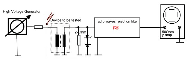
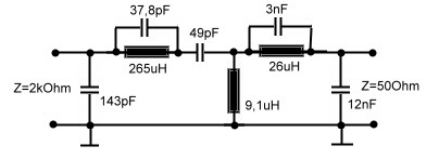
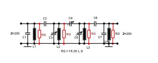
Parametric filter detects corona in molted transformers The insulation of high voltage transformers usually is measured by watching the DC-leakage current. But in molted transformers the problem of unknown tiny air bubbles exist. This bubbles my create ionization in the captive air.The corona effect may exist in a transformer for years after the high voltage breakdown will happen.The ionization bubbles can be found, watching the MHz leakage current with a scope. But this will lead to lot of mismeasurements due of added radio frequencys.To filter this radio-waves , a proper filter must used. The requirement of the filter is : Fo = 1 MHz, Zin = 1 kOhm, Zout = 50 Ohm, B =100 khz, Fig. 1 shows the measurement circuit, using a sensitive oscilloscope to watch the corona.
Fig 1 Corona measurement equipment The
Fig.2 Corona measurement filter
|
||||||||||||||||||||||||||||
|
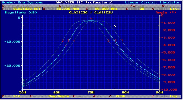
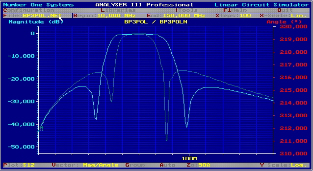
2 Pole parametric IF bandpass matches OP-AMP The above simple 2 pole parametric bandpass can be modified to be a 10Mhz IF-Filter matched to the OP-AMP in and outputs.The input of the filter has 1 Ohm to fit to the OP-output, whereas the output is resistive matched with a 100 Ohm resistor to fit the Mega-ohm input of OP-AMPs.The series connection of two or three filters between OPs give an high selectivity If-Filter. Fig 1 shows the circuit and Fig.2 the selectivity of one single filter.
Fig.2 S21 of op Bandpass (Number ONE Linear Circuit Analyzer)
|
||||||||||||||||||||||||||||
|
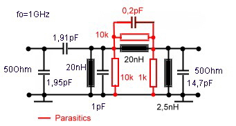
We get a simple narrow band IF filter using: The circuit is gained using Norton’s transformation and matches the output of RF-Amp to a transistor. Fig.1
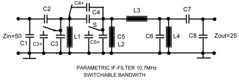
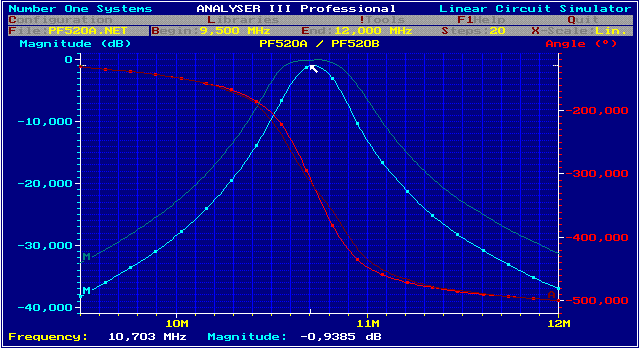
Fig. 2 Simple IF-Filter (Number ONE Linear Circuit Analyser) Bandwidth switch able If-filter To enhance the selectivity in a receiver, it is often help full to decrease the bandwidth with a switch. Fig.1 shows a IF-filter having two bandwidths. The switches can be a small coaxial relays. Their little parasitic capacitors will not affect the function of the filter to much, because on their nodes are big capacitors of 400 pF:
The component values are:
Fig.2 S12 of the double bandwidth filter (Number ONE Linear Circuit Analyser)
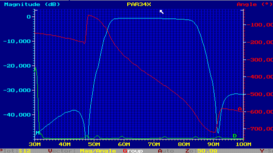
Outside band signals my disturb the digital television DVB especially at the upper frequencies of 800 Mhz. To reject this unwanted signals, a DVB-Covering filter was developed. We get a practical circuit using a the following parametric filter:
Bild 3 DVB-Covering Filter !!! Z=50Ohm
Fig. 2 S21of Pf341 (Number ONE Linear Circuit Analyser)
A Fig.1 Mixeroutputfilter-circuit
Fig.2 S21 of Mixer filter. Matching values are :S11 and S22 = 12dB.
Retour: (Number ONE Linear Circuit Analyser) A receiver-unversal-polefilter This filter is an example of filters having certain frequency poles.This example shows the high increase on rejection outside the band. We use a wave parameter filter from [3] having two resonators at Fo and two poles at frequencies near the band end. As we want high low insertion loss in the band, we add a third resonator at Fo. This filter is an universal filter to be changed for many purposes. For instance -narrow band -channel filter or high selectivity if filter. Impedance or frequency changing is easy. To change the bandwidth , the poles at band end must equally changed in percentage to broaden the band. This filter is easy to handle in a CAD-program, the three resonators are always at Fo and the poles can than be adjusted. This allows to build a bandwidth switch-able filter. Fig.1 shows the circuit for Fo =100 Mhz and Fig.2 the transmission S21setting Q=100 . Lower impedance on the input or output can be realized as it is well known , using taping of the first coil. Fig.1 Wpo2 -high selectivity universal filter
Noise measurement using a parametric if filter German Patent : DE4009076 C2 To measure the noise produced in a communication system, the bandwidth of the noise measurement device has to be limited over the bandwidth of the system. The noise power must be measured after the filter and the generated noise in the source can be computed from the ENR value: Fig:1 Noise measurement in a communication channel
The necessary data’s are: fo=140 MHz; Bandwidth 1dB =+-6 MHz, Bandwidth 3dB =+- 10 MHz , Bandwidth 20dB = +-15 Mhz. The used filter is a parametric filter having the grade of 11. The poles are : 4,1,3, Grad =11 . A PCB circuit using fixed air coils is used. To tune the filter, SMD-trimmers have been used .To manufacture a series product a lot of tolerance considerations still has to be made.The circuit up to now is shown in Fig. and the transmission S12 in Fig.4.
Fig.3 MHz noise measurement-filter
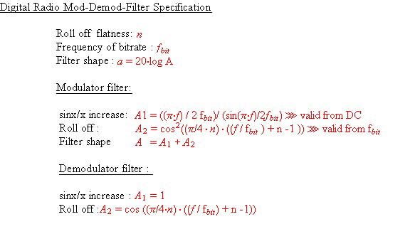
QPSK-Data Filters for digital radio Today , digital modulated communication channels are everywhere. Ignorant people may think its digital communication, using data jumps from 1 to zero, the same as digital logic . But this is not the case.We look how the communication bit’s look like and show how to design lumped RF-data filters for high bit rates. Look at two different digital bit’s, the hard jump and the soft cosines shape jump and its amplitude density. We get this density from a Fourier transformation . Fig.1. Fig.1 Amplitude density of data bits Fig. 2 shows the graphical results of this power density .The hard data bit produces power at multiples of the bit-rate. To avoid data confusion due of this unwanted power, soft square cosines bits are used in digital data communication. Fig.2 Power density of different bit’s..
Now we look to a classical specification of a filter to change the digital output bits of a QPSK-modulator into a cosines square shape. And look too, to a QPSK- demodulator specification to transform the data bit’s content , back to analog values. Fig.3. We see the shape of a very broadband low pass filter having a little sinx /x over swing before crossing the Nyquist frequency fbit. At this frequency the roll off function is working, which is a cosines square function having a variable steepness n. The demodulator filter is indeed a sinus function, written in cosines form without sin x/x increase. At Fig 4, the equations can be found: Fig.4 Digital radio mod-demod -filter specification. formulas
The Filters Mod and demod filters are both low pass filters, I use the same simple basic filter , it’s a n-pole low pass from a catalogue
[3] and select it to match approximately the specification requirements. Now how can we get the cos roll off and the sinx / x
increase? We get the roll off, by shaping the poles resonator with a resistor only damping at a certain series resonator
frequency .The sinx / x increase is very easy to get. A little differentiating resistor into the infinite pole capacitor enhances
the corner frequency over swing. This filter is much more easier to adjust than an full computed over swing filter without
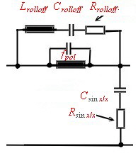
resistors, where all components my change the roll off too. Fig 5 shows one pole of the filter. Fig.6 Shows the
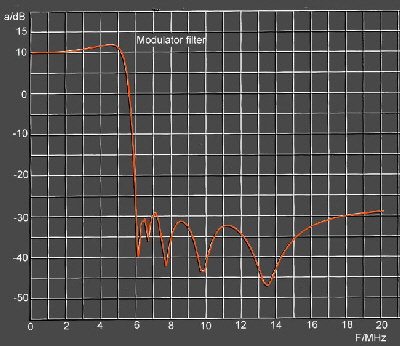
transmission of such a modulator filter, using 5 poles in series. At the 2 upper frequency s, the poles work without resistors.. Fig.5 Universal data filter pole Fig.6 Example of communication modulator filter transmission
|
||||||||||||||||||||||||||||
|
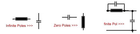
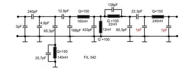
Minimum Coil Parametric 70 MHz If Filter Parametric filters need less coils than every other filter type. Here is a minimum coil broadband 70 Mhz Parametric Filter The circuit of Fig.1 is the result of computerized solving of the H(s) and K(s) equations, of a parametric filter.The components are found in a computer iteration process to nullify the equation H(s).The Circuit shows the typical C-Input of Parametric filters and has only 5 coils to get a grade of 11. Fig.2 presents the transmission . Infinit poles = 3. Zero poles =4. Finite Poles = 2. Grad = 2*2+4+3=11. Fig.1 Circuit and values of Fil342
|
||||||||||||||||||||||||||||
|
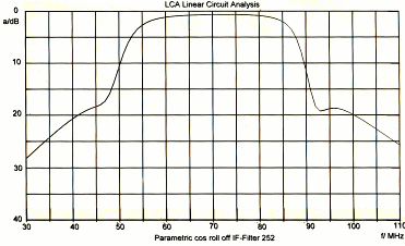
IF Parametric-Filter has cos roll off RF
Receivers for digtital data have three main sections, the RF section, including the input front end, the If section and a digital demodulator. As it can bee seen
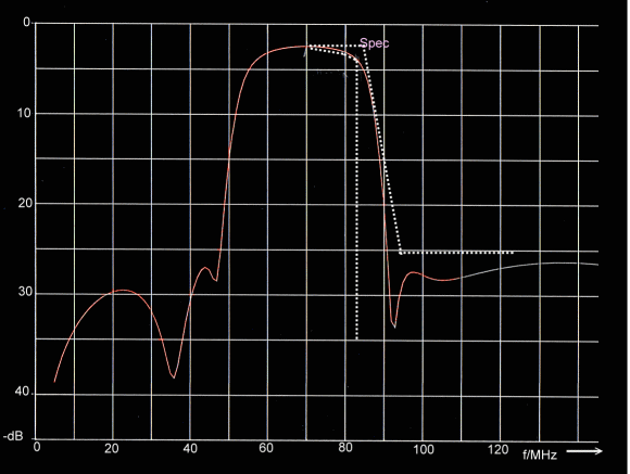
at PQSK-Data Filters for digital radio , the digital demodulator needs a low pass having a very tight specified cos roll off. This low pass, can be simplified, if the already existing IF filter has a cos roll off. . But realizing an IF Filter having this roll off; is not very easy . If we look to the filter catalogues; only very high graded Tschebischeff or Cauer filter can met this specification, but both filter circuits will not work prober at RF frequencies. Beside the specification, the filter to be designed must have a minimum number of coils having a value greater than 30nH. The here shown filter is a computer designed parametric filter having a grade of 10, see Fig.1. The values of the coils, are big enough to use fixed standard SMD Coils with a Q of >70 at 70 MHz. ( For instance Stettner, Componex or Coilcraft types) To adjust the very tight roll off specification an adjustment is used for the roll off. (R1 and R2). The poles must be adjusted, using SMD trimmers. The adjustment is easy , only the poles must be set to its frequencys. Fig.2 shows the computed filter transmission and its specification .Matching is S11= S22 =15dB;
The values are:
|
||||||||||||||||||||||||||||
|
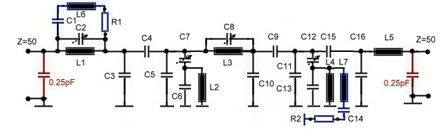
IF Parametric-Filter has cos roll off for wider specification RF Receivers for Digital data have three main sections, the RF section, including the input front end, the If section and a digital demodulator. As it can bee seen at PQSK-Data Filters for digital radio , the digital demodulator needs a low pass having a very tight specified cos roll off. This low pass, can be simplified, if the already existing IF filter has a cos roll off. Above, a very complicated filter has been shown, fulfilling a very tight specification. Here a 70 MHz bandpass is shown, having a cosines roll off, to fit in a somewhat wider specification: The electrical values fits SMD components. Adjustment is easy if the two poles are tuned to its frequencies. Fig. 1 shows the the circuit and Fig.2 the transmission.
Fig.1 Simplified Parametric bandpass having cosines roll off. The values are: C1=30pF; C2=28pF; C3=20.4pF; C4=1pF parasitic; C5=13.8pF; C6=5pF; C7=63pF; C8=120pF; C9=83pF; L1=185nH; L2=137nH; L3=185nH; L4=200nH;L5=118nH;
|
||||||||||||||||||||||||||||
|
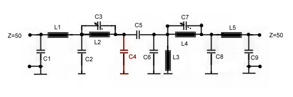
Classical Butter worth Bandpass is realized with SMD Coils Classical Radio Band-passes have been realized by means of magnetic coupled trimmed coils in a metallic housing. A better modern design, is a capacitor coupled filter having small SMD coils used as resonators. Here is an example of a 4 resonator 70 MHz broadband bandpass to be used in a telecommunication data receiver. Fig.1 shows the circuit. As the SMD coils are not trimmed at all, three adjustment SMD capacitors are used to compensate the 5 % delivery tolerances of the coils. Fig 2 shows the S12 transmission at 200 Ohm matching, S11/ 22 is 20 dB. On a PCB, the coils must be placed between small flat metal shields, soldered on the PCB, to prevent magnetic coupling. The circuit values are :
As the components are very tight selected, adjustment time of the filter is only a few minutes.
Fig.1 Classic Butter worth bandpass data filter
Fig.2 Tuned bandpass (Number ONE Linear Circuit Analyzer) The numbered shapes are : (S12 is matched gain) :
Return : |
||||||||||||||||||||||||||||
|
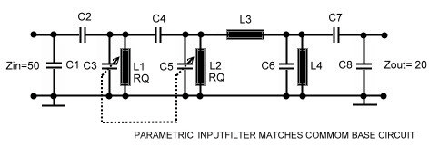
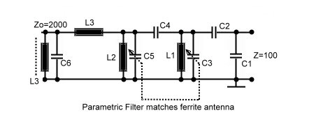
Parametric filter matches receiver input Show IF-filter The IF- Filter shown above in this site can be transformed using Norton’s transformation, to match input antennas to a RF input-amplifier. To tune this grade 7 filter, only two variable capacitors are necessary. The matchings are:
Fig.1, 50 Matching of a 50 antenna to a common base transistor The values are: C1=8pF; C2=15pF, C3=27pF; C4=1,5pF; C5=40pF; C6=5pF; C7=40pF;C8=1pF; L1=33nH;L2=33nH;L3=300nH; L4=100nH; (High Q SMD Coilcraft Aircoils) Fig.2 S21 at frequency tuning . C3 from 20 to 28 pF and synchrony C5 from 30 to 40 pF
Fig.3 Matching of a ferrite antenna The values at fo = 80 Mhz are: C1=15pF; C2=30pF, C3=1pF; C4=2pF; C5=25pF; C6=25pF; L1=200nH; L2=160nH; L3=4uH; L4=180nH; The resonance frequency of L3 must be >3fo, therefore this coil must be realized using a high permeability RF-Ferrite, to need only 3 to 7 turns. Component Values can be scaled by fo1/fo2 to change fo. Return :2 |
||||||||||||||||||||||||||||
|
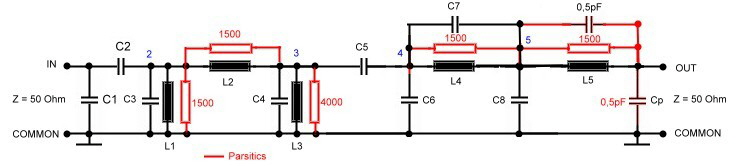
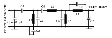
Parametric Data IF Bandpass has 2 finite poles Parametric Band-passes with finite poles are a good choice for broadband data filtering .As an example, a 2 finite pole bandpass has been computed using a FORTRAN Program . The circuit was found by means of nullifying the roots with circuit elements in an interactive process. The program finds many solution circuits which all solves the roots.The designer has to decide which circuit has to be used. Fig 1 shows the chosen circuit.The output impedance is set to the 90 Ohm to optimize PCB wiring. Fig.2 shows the computed S21 transmission values for broad and narrow-band. If the infinite pole frequencies are changed using C2 and C6 synchronously, the bandwidth may be changed up to 30 % .
The Component values are:
Fig.2 Transmission of Broadband parametric bandpass (Number ONE Linear Circuit Analyzer)
|
||||||||||||||||||||||||||||
|
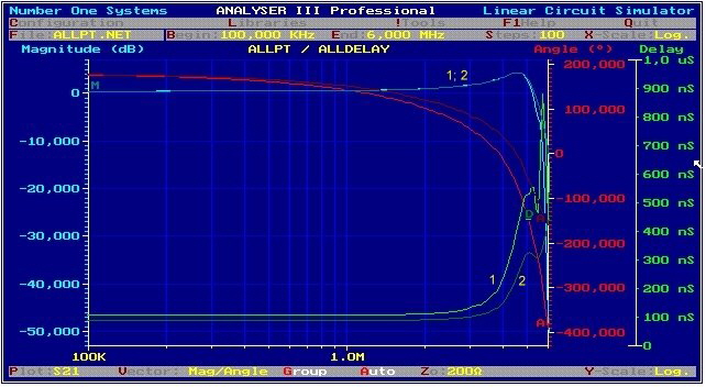
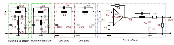
QPSK-transmitter low-pass with groups delay compensation Here is an example of the application of a run time equalizer application to compensate groups run time in a digital communication modem. The groups runtime which will be compensated is the delay of a low-pass in a QPSK transmitter modulator , having a sinx/ x part , befor the roll off frequency. This low-pass is shaping the bits but it should not delay it. Fig.1 shows the transfer S21 of the filter. We see at 5Mhz a sinx/x increase of 0.5dB followed by a very steep roll off. The phase of the combination of sinx/x increase and sharp roll off, produces a lot of groups run time which must be compensated . The run time behavior of of the low-pass with and without groups run time compensation, shows fig.2. The circuit of the low-pass has 5 sections (Fig.3), 2 groups run time equalizer, and 2 low-pass poles and a sin x/x circuit using the combination of series and parallel resonator driven by means of a RF Op-Amp. The equalizers are standard 45 degree circuits , explained at : Go to run time equalizer circuits:
Fig.3 Circuit of QPSK transmitter lowpass
|
||||||||||||||||||||||||||||
|
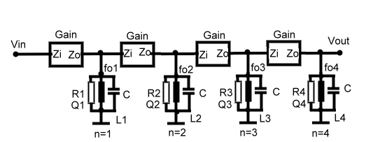
Broad-band IF-filter realized by means of single resonators between FET’s or tubes The broadband filters shown above, are the outcome of complicated computer filter software including NORTON transformation. Here is a very simple method to realize an other type of broadband band-filter. Such simple filters have been used in the earlier years of electronics. The only thing we need for calculation is a pocket calculator. Fig. 1 shows the basic block diagram of the filter. We see between two amplifiers, which have a very high input and output resistance, one detuned L C resonator. This amplifier-resonator circuit is connected in series n times and it is assumed, that Zi and Zo are very high. The amplifier can be a FET or a Tube. If the impedances are low, they can be transformed, using coil-taps. The gain must be stable fixed, using a feedback circuit.
First we define the parameters :
In case of z = 4, the resonator values for a butter-worth shaped filter can be found using the following equations:
The same filter can be constructed with tschebischev behavior if the following parameters are used:
Fig.1 shows, how the single resonators are added together.
|
||||||||||||||||||||||||||||
|
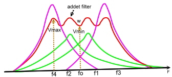
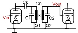
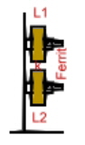
The classical radio bandpass filter. This article is written for tube radio fans, for understanding the classical radio LC, I F-band filter, which are not used any more in todays radios. This bandpass, was realized , using two high Q Coils as of part of two resonators, which are coupled using the magnetic field of the coils. Fig.1 shows the mechanical arrangement. The coils have been placed on two small plastic tubes with ferrite adjustment screws. Turning this screws, the mitt-frequency of the resonators can be changed. The distance between the coils determines the bandwidth of the bandpass. This two resonators are connected between tube amplifiers as fig.2 shows. Fig.1 mechanical filter design.
Fig.2 circuit of classical radio bandpass The following parameters are valid:
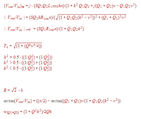
The main formulas are:
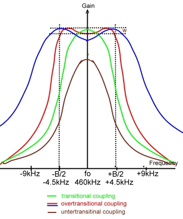
At Fig.3, 460 kHz Radio IF- Bandpass curves depending on different coupling factors are shown.The stop band attenuation at 9kHz must be as high as possible!
|
||||||||||||||||||||||||||||
|
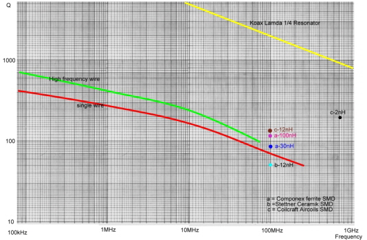
Computing
of an electronics filter is one thing, realizing the hardware, is another, because of coils quality and self-resonance. Fig.1 shows this coil losses. Before build up the hardware, the filter should be tested with the coil-datas and its parasitic values, in a CAD Program.
The losses have the fol
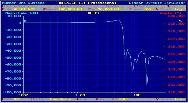
We see in the frequency range between 100 MHz and 2 GHz, only air coils and coax resonators have high Q values. . As coaxial resonators with high Q values are very bulky, the only solutions are air coils especially SMD air coils. That is, the filter tuning must be made with capacitors. 140 MHz Broadband Parametric-IF Filter for a Digital Modem. German Patent DE 4009075 C2 A 140 MHz Parametric-Bandpass Filter for a Receiver Data Modem has been developed. The Input matched Filter circuit has been found, by using “ Saals”* Formulas in a Fortran Program for Zin =50Ohm,. The output of 1.5 Ohm then was matched using a “ Norton” transforming Software. The testing has been made using “Compact “ linear analysis. *SAAL, “THE CATALOG OF NORMALIZED LOW PASS FILTERS”;
Parametric-Filter-Components are:
Simplification of the 140 MHz Broadband Parametric-IF Filter for a Digital Modem. German Patent DE 4009076 C2 If C10, C12, L8 of Fig.1 are set to 0, C11and L9 to infinite, the Norton Transforming program tries to find positiv finite other values. After working a few hours, with norton, we get a simpler circuit. Fig.4 . The out of band rejection is even greater. Fig.5.
Fig.4 Simplified 140 MHz parametric bandpass circuit and values
Fig.5 S21, S12 of the simplified parametric 140 MHz bandpass
Fig.6 S11,S22, of the simplified parametric 140 MHz Bandpass Practical realisation of the parametric filter As the capacitor data shoes, all capacitor values to ground have been made with the Norton-programm relatively large. Therefore, the Filter-PCB has a full grounding layer. The actual C values than must be smaller than the parasitic values from the board. As Fig 4 shoes, the filter has a dimension of 6 cm * 2cm. To get the ground really cold I have soldered two angel plates along the board at the ground side. To prevent parasitic inductance the string from input to output must be made very broad. The hard ware was tested an I got nearly the computed values. Fig. 7 Test-PCB of the parametric Bandpass filter, (about real) size.
Return :
|
||||||||||||||||||||||||||||
 Filter is a transforming parametric circuit using lumped components rare then an OP-active filter which could be damaged from high voltage sparks. Fig.2. Fig.3 shows S21 .
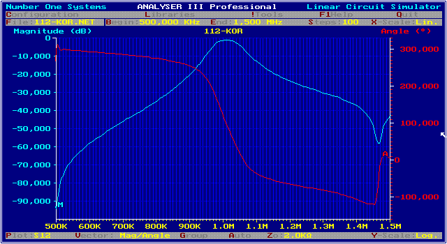
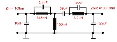 Fig.1 OP-AMP bandpass
 Fig. 1 IF-Filter 10 MHz
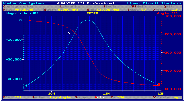

 Mixer must work into some resonating device to gather the wanted mixing products. A small filter can do this job, but it
must be properly matched. We use:
Mixer must work into some resonating device to gather the wanted mixing products. A small filter can do this job, but it
must be properly matched. We use: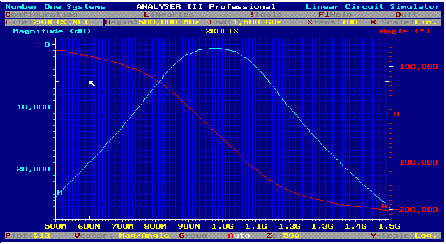
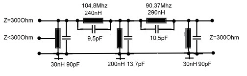
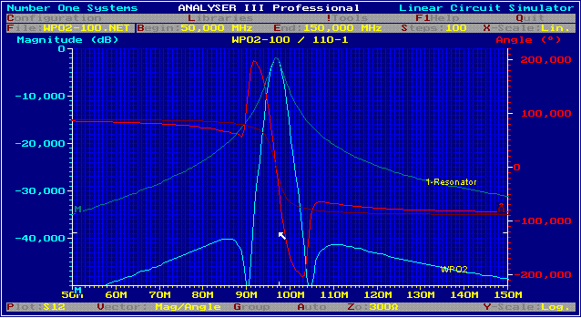
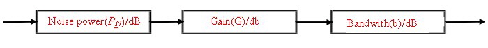
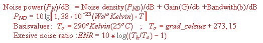
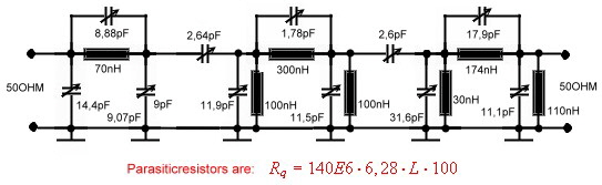
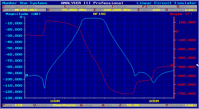
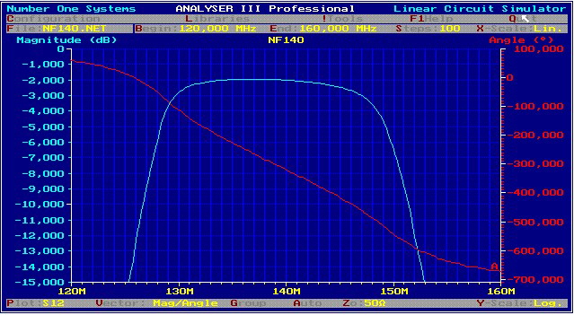
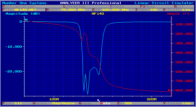
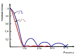 Fig. 3 Filter specification of digital radio mod-demod filter
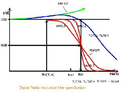
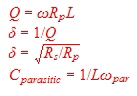 lowing formulas: