|
Lechler’s Website: |
|||||||
|
|
|||||||
|
|
|||||||
 |
|
Engineering - Electronics - Content :
|
|
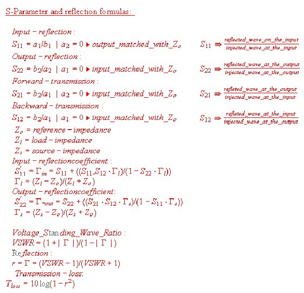
S-parameter are very practical and have outset classical parameter like VSWR and reflection. Here are the basic equations of S-parameter and it’s transformation formulas to impedance, reflection and standing wave ratio. S-parameter are widely used in electronic CAD programs in the popular touchstone format. We can type a touchstone format file from measured S parameter values.Using this files we can compute Y to S-parameter values. >>>go to S-parameter example
|
 |
|
S-parameter touchstone file format S-parameter catalog or measurement values can be written in a touchstone cad-file to be used in CAD-programs. The green text must be written in a ASC2 DOS text-file.
frequency S11 S11angle S21 S21angle S12 S12angle S22 S22angle
|
||
|
Y-parameter touchstone file format Y-parameter catalog or measurement values can be written in a touchstone cad-file to be used in CAD-programs. The blue text must be written in a ASC2 DOS text-file.
frequency S11 S11angle S21 S21angle S12 S12angle S22 S22angle
|
||
|
Y-parameter to S-parameter equations Y-parameter can be expressed as S-parameter and vice versa. Some older component catalogues only show the y parameters. To avoid tedious computing , one can create a Y-block to be analyzed in a CAD-program and save the results as S-parameter file. |
||
|
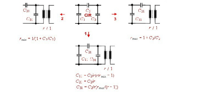
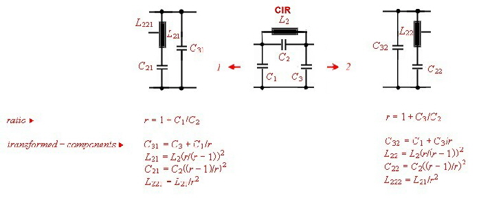
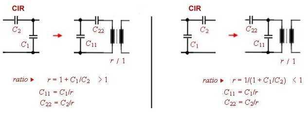
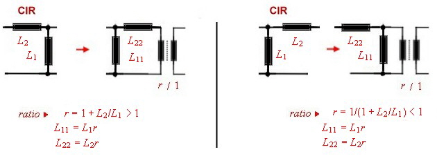
Norton transformation of circuits The circuit of a lumped filter can be simplified ,, using Norton’s
transforming equations . That means a part of the circuit can be replaced by an other circuit and a ideal transformer. The transformer then must shifted to the input or output of the circuit and removed by changing
the actual input or output impedance. An other way to free the changed circuit from the transformer, is to transform 2 circuit parts ore more having the opposite transforming ratio. The transformer than can be
canceled if they are directly connected.. Go to Norton’s example. At Fig.1-5 the CIR named circuit parts of a filter can be replaced by the transformer circuits 1...2...3...and / or transformed with the transformer ratio.There are other possibility’s of Norton’s transformation but they are not shown here.
Fig.2 -5 Nortons transformation
|
|
Each Electronic book has an epsilon table of materials, but the constants of PCB-materials like FR4 or Pertinax or Araldid, you never will find. Here are the epsilon values of popular RF-materials:
|
|
|
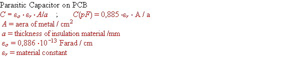
The capacitance of a PCB-capacitor Designing RF-circuits means to be aware of parasitics. Parasitic capacitors can be estimated using the basic formulas: |
 |
|
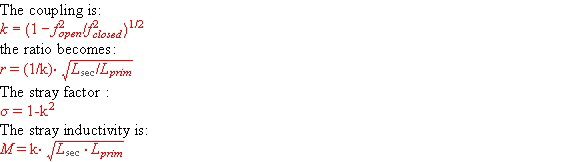
Measure the RF-transformer coupling: We have two coupled RF-coils and want to know the coupling. Here is how we can measure it:
|
|
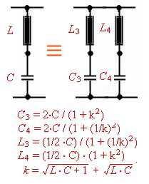
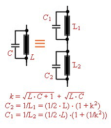
Replace two resonators in lumped filters Lumbed RF- Filter circuits from a catalogue, often seems to be very complicated. Here are the formulas to replace a two resonator circuit into a one resonator circuit. ( only valid for narrowband circuits) Fig.1 Replacement of two series resonators
|
|
Basic Transformation of wave lines Wave lines come out in different mechanical configurations , either as Coax-cables, lines on a PCB or ceramics (Micro Strip) ,Parallel lines, Twisted wires and special Strip lines. Each type has its one impedance Z. The impedance of all this configurations are different and depend on the material, and the
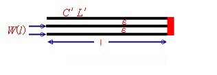
mechanical size. The basic transformation formulas for all configurations are the same: A complex output resistor will be transformed to an other complex resistor at the input of the line. Fig.1
The values of this input resistor can be found, either by means of th
Fig.1 Transforming Wave line equations
Fig.2 Basic wave line transforming formulas The shorted wave line resonator
Fig. 3 Resonance condition with short termination
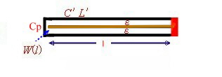
The capacitor input, wave line resonator This resonator has an paralleled capacitor at the input. Fig.5 This is the typical filter resonator. The capacitor Cp is used to
adjust the resonator frequency . The resonance formula shows ringing at frequencies different from the harmonics to the basic resonance.
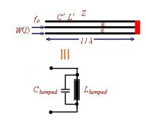
Fig.5 C-loaded Resonator The C or L loaded wave line Resonator
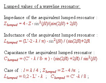
The lumped resonator values of wave lines
Fig.6 Equivalent lumped circuit
Fig.7 The values of the lumped circuit Link>>> Go to example of line resonator
|
|||||||
|
The Surface Resistance of metals at RF-Frequencies RF- losses in wires, filters, resonators, PCB-connections a.s.o., depends on the RF-skineffect at the surface of the used metals. The
skin effect in the RF-range is defined as resistance at a certain area A. The skin effect factor Rho ’ For instance , R’ is the loss per cm of a coax cable having a an impedance of Z = SQR(L’/C’). R’ must be used to calculate the Q-values of wave line resonators. The values of the specific surface resistance are shown in a diagram. Fig.1 shows the normalized factor Rho’ for different materials as silver, copper, aluminum, and brass in the RF-frequency range from 300 kHz to 30 Ghz
|
|||||||
|
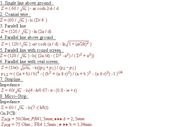
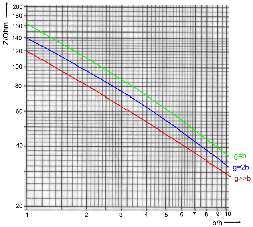
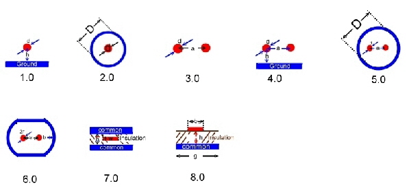
The impedance of a wave line depends on the mechanical dimension and the epsilon value of their insulation. Fig.1 and 2 presents the impedance equations of following wave lines:
Fig.1 Impedance equations
Fig.3 Z of Micro-Strip at epsilon air =1 (for other insulation materials Zx = Zair/SQR(Epsilonx) ; (g look 8.0) Link >>> Go to epsilon values
|
|||||||
|
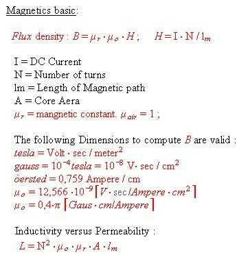
:Magnetics basic equation , and the factors between’ Gauss’ ; ‘Tesla’, ‘Öersted’ and ‘V*s/m*m’, The basic magnetic equation often has been forgotten . Remember the induction in a magnetic core Fig.1 see the factors between’ Gauss’ ; ‘Tesla’, ‘öersted’ and ‘V*s/m*m’, and go to an example of magnetic: >>> go to magnetic example >>>> t.b.c. Fig.1 Basic Magnetic formulas |
|||||||
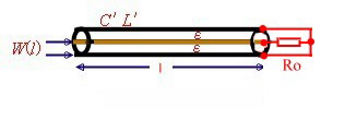 e formulas, shown at Fig.2, or using a Smith Chart :
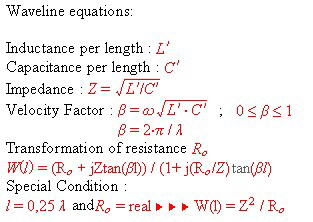
 As the length of the line is important, multiples of the length to lambda factor, make the conditions, where the line will resonate. Either as
parallel or series resonator. Using this length, we get new conditions especially if the line is shorted on the end. Fig.3 shows the resonant
conditions for the shorted line. The transformation equation is simplified to :
As the length of the line is important, multiples of the length to lambda factor, make the conditions, where the line will resonate. Either as
parallel or series resonator. Using this length, we get new conditions especially if the line is shorted on the end. Fig.3 shows the resonant
conditions for the shorted line. The transformation equation is simplified to :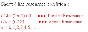
 . The resonance frequency can be found using a little computer program on a pocket computer to solve
following equation:
. The resonance frequency can be found using a little computer program on a pocket computer to solve
following equation: